Material
The slides are extracted from my PhD proposal. For the official conference presentation slides, please refer to the official 2023 AISTATS website.
Notation
Note that a set of states, \(\mathcal{S}\) and a set of actions, \(\mathcal{A}\), which might be infinite, i.e. \(S=|\mathcal{S}|\leq\infty\), \(A=|\mathcal{A}|\leq\infty\).
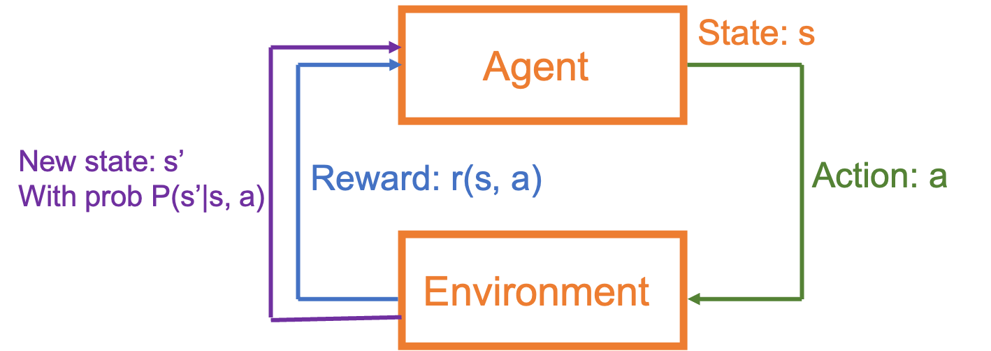
Task
Given a model of the environment, how many transitions do we need to observe for finding an ``near’’ optimal policy with high probability.
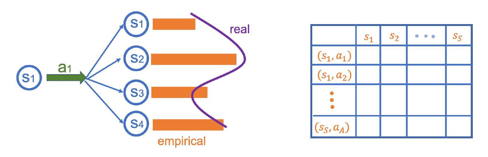
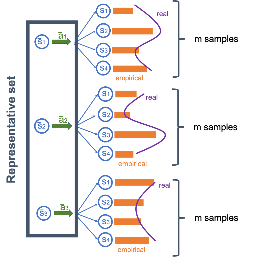
According to above figure, given a state-action pair \((s,a)\), we hope to estimate the transition probability to next state. That is, we need to fulfill this table with size \(SA\times S\). However, if there is infinitely many state action pair, then what can we do?
Introduction
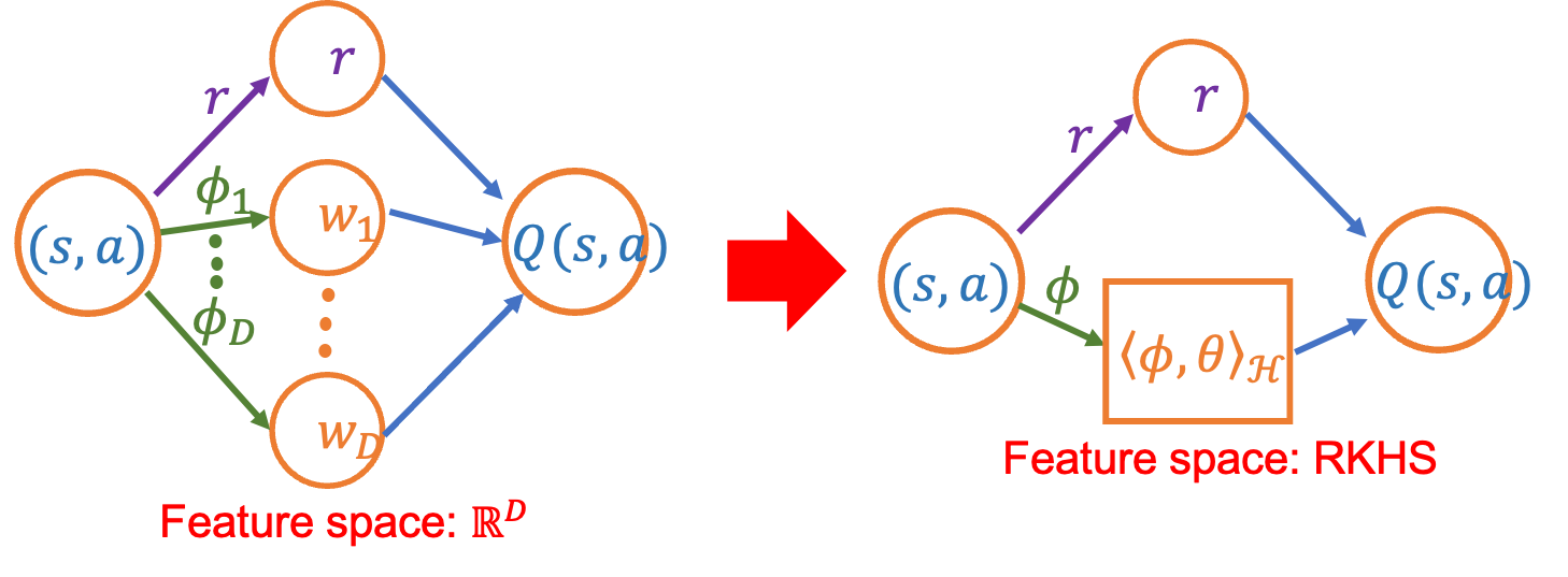
Linear property To deal with large state action pair, traditional method is to apply linear property, such as Yang & Wang (2019), which still focus on finite state action pair. The idea is as following given a \(D\)-dimensional feature space, the feature map \(\phi:\mathcal{S}\times\mathcal{A}\rightarrow \mathbb{R}^D\). Exist \(\psi:\mathcal{S}\rightarrow\mathbb{R}^D\) such that
\[P(s'|s,a)=\phi(s,a)^\top \psi(s')=\phi_1(s,a)\psi_1(s')+\cdots+\phi_D(s,a)\psi_D(s')\,.\]Since \(Q(s,a)=r(s,a)+\gamma \sum_{s'\in\mathcal{S}}P(s'\vert s,a)V(s')\), then exist a vector \(w\in\mathbb{R}^D\), such that
\[Q_w=r(s,a)+\gamma\phi(s,a)^\top w.\]Moreover, we write \(\sum_{s'\in\mathcal{S}}P(s'\vert s,a)V(s'):=\gamma PV(s,a)\).
Kernel setting Now, we generalize the finite dimensional feature space to infinite dimensional space (reproducing kernel Hilbert space) via kernel method. Since reproducing kernel Hilbert space (RKHS) belongs to \(L^2(\mathcal{S}\times\mathcal{A})\) so that we can generalize to infinite state action pair.
Related Literature
The following is listed some algorithm and their sample complexity upper bound. Note that \(\tilde{O}\) stand for ignoring the \(log\) term.
-
Tabular setting, finite state action pair in Sidford et al. (2018). The sample complexity upper bound is \(\tilde{O}\left(\frac{SA}{(1-\gamma)^3\epsilon^2}\right)\). Actually, the theoretical lower bound of sample complexity is \(\tilde{\Omega}\left(\frac{SA}{(1-\gamma)^3\epsilon^2}\right)\).
-
Linear transition probability setting, finite (large) state action pair in Yang & Wang (2019). The sample complexity upper bound is \(\tilde{O}\left(\frac{D}{(1-\gamma)^3\epsilon^2}\right)\). The step of this method is choose the representative set first, and obtain the sample from the representative set to estimate the transition probability.
Methodology
I replace the finite dimensional feature space by RKHS in order to deal with infinitely many state action pairs. TBA, when I finish and publish the result.
Reference
- L.F. Yang & M. Wang, Sample-Optimal Parametric Q-Learning Using Linearly Additive Features., (2019).
- Z. Yang, C. Jin, Z. Wang, M. Wang & M.I. Jordan, On Function Approximation in Reinforcement Learning: Optimism in the Face of Large State Spaces., (2020).