Predict survival of the people on Titanic by ML

Introduction

We hope to predict whether the people on Titanic is survival or not. This data is from website ''kaggle''. Actually, there are lots of method solve this problem and make a good prediction, for example, logistic regression. Hence, in this project we just predict it by the tool which we learned in the ML class.

Feature Engineering

In this section, the basic feature engineering will be introduced. The following analysis provides a simple base for prediction.

Gender and age

The following figure show the survival in different gender and age. ori img

Figure: Comparison the survival between male and female.

We can compute that the following table. If we set males are perished and females are survival, then the accuracy will be 0.7655. It provide a useful criteria for other classified machine. Then, we define another parameter "child", which is defined as age less than 10.

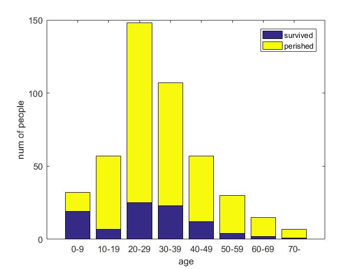
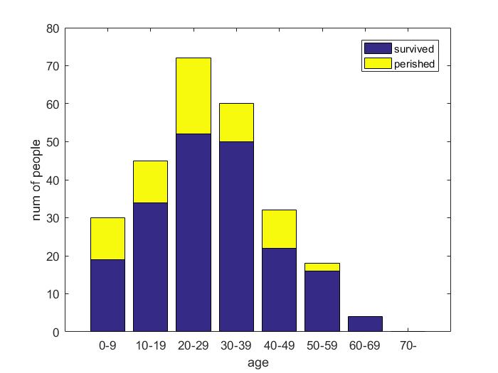
Parameter	Female	Child
Accuracy	0.7655	0.7703

Family size

Define family size is SibSp plus parch. The survival rate is high when family size is 4 or 5. We think it can provide another parameter. ori img

Figure: Comparison the survival between different number of family.

Parameter	Female	Child	Female, Child and Family size
Accuracy	0.7655	0.7603	0.7464

Fair and Pclass

Now, we see the relation between Fair and Pclass. It seems that there are no obvious relation between them. ori img

Figure: Comparison the Fair and pclass.

However, by following table, the survival rate is much different between different Pclass.

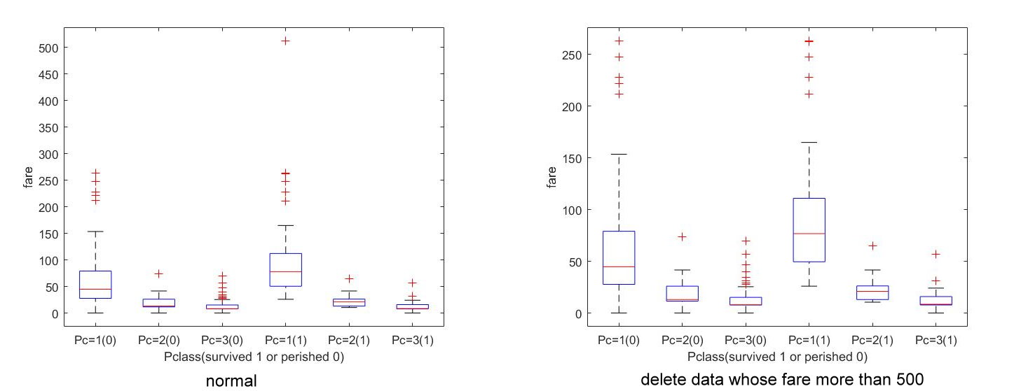
Pclass	1	2	3
number of survival people	136	87	119
number of perished people	80	97	372

Logistic Regression

If we choose the original parameter, by logistic regression, the following p-value can be gotten. We can deduce that survival have low relation with Parch, Fare and Embarked.

Parameter	Pclass	Sex	Age	SibSp	Parch	Fare	Embarked
p-value	0.0000	0.0000	0.000	0.0015	0.3199	0.2703	0.4230

Then, we choose the previous artificial parameter, e.g. child, family size and fare times Pclass.

Parameter	Pclass	Sex	Age	SibSp	Family size	Fare*Pclass	Child
p-value	0.0000	0.0000	0.000	0.1760	0.2452	0.1337	0.9861

Hence, the following two combination of parameter are chosen $$\mathcal{A}=\{Pclass, Sex, Age, SibSp\}$$ and $$\mathcal{B}=\{Pclass, Sex, Age, SibSp, Fare*Pclass\}$$

PCA

We use PCA to reduce dimension of original original, i.e. Pclass, Sex, Age, SibSp, Parch, Fare, Embarked. Then, how many eigenvector is taken is chosen by logistic regression.

eigenvector	1st	2nd	3rd	4th	5th	6th	7th
p-value	0.0000	0.0000	0.0000	0.0035	0.0021	0.9986	0.0000

Hence, let $\mathcal{C}$ be the first 2 vector, $\mathcal{D}$ be the first 3 vector and $\mathcal{E}$ be the first 3 vector and the last vector.

Experiment

Because we could check answers only few times, we choose the radial bump kernel which is recommended on website, first.

1-norm Soft margin SVM with radial bump kernel

Train an 1-norm soft margin SVM classifier using the radial basis kernel. That is,

$$\max_{\alpha}\sum_{i=1}^{l} \alpha_{i}-\frac{1}{2} \sum_{i=1}^{l} \sum_{j=1}^{l} \alpha_{i} y_{i} \alpha_{j} y_{j} K\left( x^{i}, x^{j}\right)$$

subject to $0\leq\alpha_j\leq C$ and $\sum y_i\alpha_i=0$, for some $C$. Note that this inequality $0\leq\alpha_j\leq C$ is called the box constraint. Now, the following table is show the accuracy of SVM with $C=1$ and gauss kernel scale $\sigma=1$.

method	origin	$\mathcal{A}$	$\mathcal{B}$	$\mathcal{C}$	$\mathcal{D}$	$\mathcal{E}$
accuracy	0.76555	0.77272	0.76794	0.70813	0.77511	0.77511

Only method $\mathcal{C}$ is not higher than just use female to predict. Then, we focus on method $\mathcal{B}$, i.e. {Pclass, Sex, Age, SibSp, Fare*Pclass} and classify them by other method in our class.

Tuning procedure

Now, we focus on method $\mathcal{B}$. Hope to find a better box constraint $C$ and Gaussian kernel scale $\sigma$. First, the 30-fold cross validation is used. The tuning procedure is shown as following.

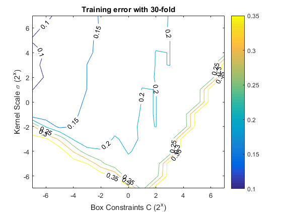
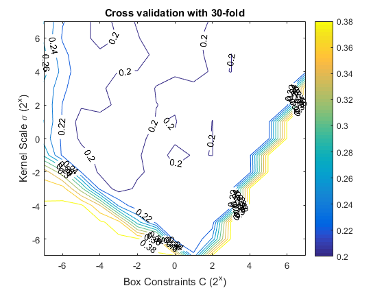
Figure: The left figure shows training error and the right figure show validation error during the tuning procedure.

Now, we choose some pairs of $(C, \sigma)$.

$(C,\sigma)$	(4, 0.25)	(2, 0.25)	(1, 1)	(0.5, 4)
training error	0.1616	0.1627	0.1874	0.1998
validation error	0.1886	0.1886	0.2020	0.1998
testing accuracy	0.76555	0.76555	0.77272	0.77272

ROC curve: compare two model

The parameter $(C=1, \sigma=1)$ and $(C=0.5, \sigma=4)$ have the same test accuracy. We desire to tell the different between two model so we choose receiver operating characteristic curve.

True Positive Rate (Recall, Sensitivity): how many correct positive results occur among all condition positive samples.
False Positive Rate: how many false positive results occur among all condition negative samples.

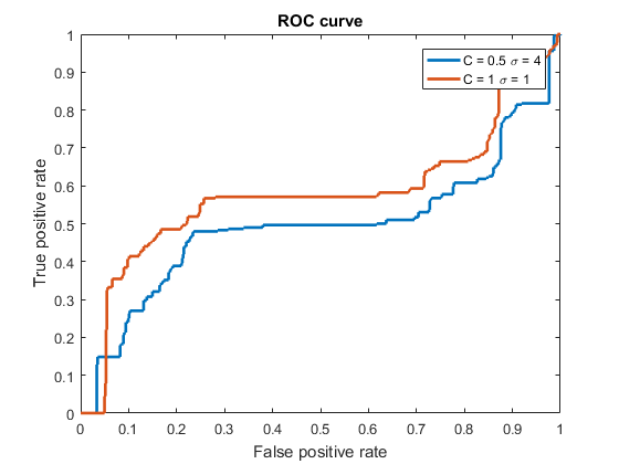
Figure: Comparison the Fair and pclass.

The AUC of $(C=1, \sigma=1)$ is 0.5799 and the AUC of $(C=0.5, \sigma=4)$ is 0.4868. Hence, choosing the parameter $(C=1, \sigma=1)$ is better.

Smooth SVM (SSVM)

In class we learned SSVM, so we download SSVM matlab code from website “http://dmlab1.csie.ntust.edu.tw/downloads/”. Then, we got accuracy is 0.76555.

Result

Now, we use a complicated method (SVM) to predict whether the people are survival or not. Hence, the t-test is used to explain whether SVM method is better than just classifying by gender.
Set 30-fold. Let two method is same ($\mu=0$) to be null hypothesis ($H_0$) and $\mu\neq 0$ to be $H_1$. Choose significant level $\alpha=0.1$. Now, compute

$$t=\frac{\bar{d}}{\sigma/\sqrt{n}}=-1.3499$$

Moreover, $p$-value is 0.0945. Hence, we cannot reject null hypothesis. My SVM is not significant powerful in this case. Futhermore, $t_{0.95}(29)=1.699$ and $t_{0.90}(29)=1.311$.

References

Yuh-Jye Lee, Machine Learning Lecture Note, NCTU(2017)
Eric Lam and Chongxuan Tang, CS229 Titanic–Machine Learning From Disaster
Yuh-Jye Lee and Olvi L. Mangasarian. SSVM: A Smooth Support Vector Machine for Classiﬁcation

Acknowledgements

Thanks my classmates Yuehchou Lee and Chunyen Huang. I would like to thank Dr. Lee for the guidance and encouragement.